This is part two of a series on Fourier analysis and intuition.
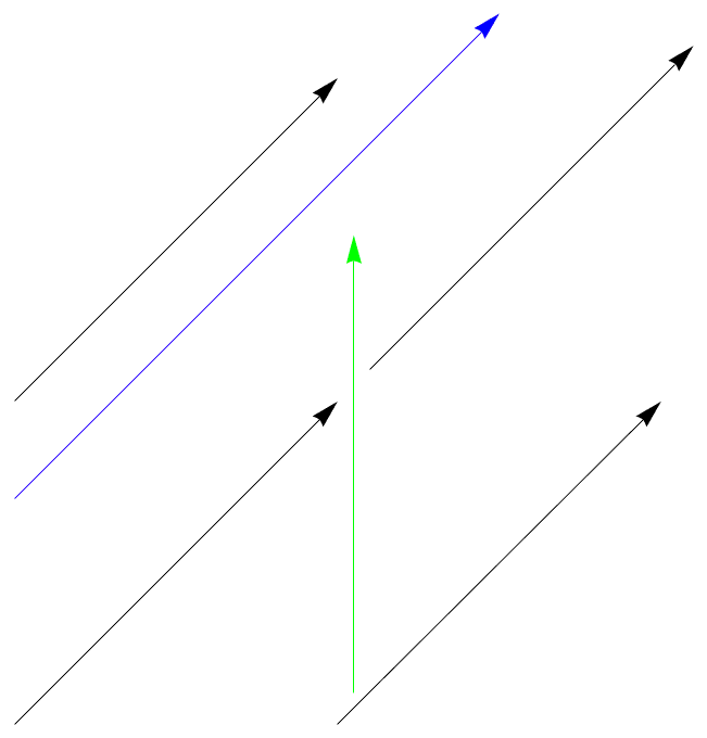
In the intro post to this series I promised to explain how Fourier analysis is similar to the geometry of shadows but noted I would first have to talk about geometry and shadows to explain it. Now I’m getting started on talking about geometry, and the first concept I want to explain is that of a vector. A lot of different mathematical objects with similar properties are called vectors and this series is essentially about exploiting that analogy as an intuition pump. So I’ll first discuss geometrical vectors that can be understood fairly intuitively. In that sense a vector is basically a class of arrows of the same length and direction. Here’s an illustration of the concept:
Or maybe it’s modern art and worth a million dollars
The black arrows all represent the same vector. The green arrow belongs to a different vector though, because it points in a different direction, even though it has the same length. The blue arrow represents a third vector, because it shares the direction of the black ones but not the length.
Another way to think of it would be as a displacement or movement instruction like “six feet to the right”, which doesn’t depend on the starting point and is different both from “ten feet to to the right” and from “six feet under”.
Now on to things we can do with vectors. If we have two of them we can add them getting a third one. This is done by pinning an arrow representing one vector to the end of an arrow representing the other one and then connecting first one’s starting point to the second ones end point. I drew you a picture of that:
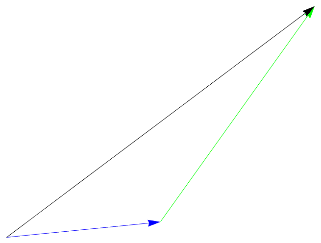
Here I added the blue and the green vector giving the black one. (The colors are for illustration, the concept of a vector is colorless.) If you think in terms of displacements you can imagine it as a temporal succession: first one yard to the left, then one yard to the front, the sum is what would have led you there directly.
We can also give our vectors names. Often vectors and numerical variables are distinguished typographically so that they don’t get mixed up. One popular way to do this is to draw a little arrow over letters representing a vector and this is the convention I will be following. So, for example, in the addition picture above we could call the blue vector \(\vec x\), the green one \(\vec y\) and the black one \(\vec z\). Then we can write the addition as an equation: \(\vec x+\vec y=\vec z\).
One might wonder why this operation is called addition. The word addition already means something for numbers, isn’t it an abuse of language to recycle the word for a different operation? Well sort of, but there’s a good excuse: This addition is similar to real addition in obeying similar rules.
For example, if you have any two vectors \(\vec x\) and \(\vec y\), it is true that \(\vec x +\vec y=\vec y + \vec x\). To put this in pompous words, vector addition is commutative.
With a third vector \(\vec z\) we also get \(\left(\vec x +\vec y\right)+\vec z=\vec x +\left(\vec y +\vec z\right)\). In math-speek vector addition is associative.
We can also introduce a zero vector \(\vec 0\). On the movement picture you can imagine it as “just stay where you are”. In the arrow picture it’s a borderline case, because it’s just no arrow at all. Anyway, if we do that, \(\vec 0\) behaves a lot like the number \(0\): For any vector \(x\) we get \(\vec 0+\vec x=\vec x+\vec 0=\vec x\). In math-speek we express that as vector addition has a neutral element.
Finally, for every vector \(\vec x\) we can find a vector \(-\vec x\) so that \(\vec x +\left(-\vec x\right)=\vec 0\). We abbreviate this as \(\vec x-\vec x=\vec 0\). In the movement picture \(-\vec x\) is just the movement that undoes \(\vec x\). In the arrow picture it would be the arrow that points from the end point back to the starting point. In mathematical language, every vector has an additive inverse.
Don’t sweat the details, the main point is this: vector addition is called addition by a legitimate analogy to normal addition because it obeys basically the same rules.
Another thing we can do with vectors is multiply them by numbers. In the arrow picture we do this by multiplying their length by the numbers. So if we have a number \(a\) and a vector \(\vec x\), \(a\vec x\) points into the same direction as\(vec x\) but is\(a\) times as long. In the movement picture it could me imagined as repeated movement. For example, moving a yard to the right five times is the same as moving five yards to the right. We call this operation scalar multiplication. (Scalar is basically a fancy word for number.)
Scalar multiplication, too, is analogous to normal multiplication by sharing some of it’s rules. The details won’t be very important for what I wish to explain, so I’ll just state the rules for completeness. For any given numbers \(a\) and \(b\) and any given vectors \(\vec x\) and \(\vec y\) we have:
$$a\left(b\vec x\right)=(ab)\vec x$$
$$a\left(\vec x+\vec y\right)=a\vec x+a\vec y$$
$$(a+b)\vec x=a\vec x+b\vec y$$
$$1\vec x=\vec x$$
So that’s how geometrical vectors work. But they aren’t the only kind of vectors. Other objects are called vectors for being similar to them. And the similarity consists in obeying the same rules. Any set with two operations that obey the rules of vector addition and scalar multiplication is, by definition, called a vector space. Or, to say the same thing more pompously, these rules are the defining axioms of vector spaces. This is often useful, because it allows transferring some intuitions from arrows to much more complicated objects.
So what other kinds of objects are vectors? Well the example that will turn out important for this series is functions. If we have functions \(f\) and \(g\) and a number \(a\), we can simply define an addition by \(\left(f+g\right)(x)=f(x)+g(x)\) and a scalar multiplication by \((af)(x)=af(x)\). In other words just perform the addition and multiplication on the function’s results. It turns out that these operations fulfill all the axioms. So, in a way, functions are just like arrows.
Later on that will allow us to transfer some intuitions from arrows to functions. But I’m getting ahead of myself. First my next installment will have to discuss some other things that can be done with arrows.